
The Earth undergoes continuous bombardment by cosmic rays from the galaxy. These are atomic nuclei (mainly protons) traveling through interstellar and interplanetary space at relativistic speeds. The net flux of cosmic-ray energy intercepted by the Earth is low and roughly equivalent in intensity to visible starlight. However, the energy of each particle is very high, averaging several billion electron volts (the kinetic energy of a gas molecule at 10 000 oK is about one electron volt). Cosmic rays can, therefore, interact strongly with matter.
Cosmic rays generate unstable nuclides in two principal ways: by direct bombardment of target atoms (causing atomic fragmentation or ‘spallation’), and by the agency of cosmic-ray-generated fast neutrons. The latter is produced by the collision of cosmic rays with target molecules and slowed by further collisions to thermal kinetic energies. These ‘thermal’ neutrons are able to interact with the nuclei of stable atoms, causing transformations to radioactive nuclei. The ‘cosmogenic’ nuclides thus produced can be used as dating tools and as radioactive tracers.
Terrestrial cosmogenic nuclides (‘TCN’) are produced in two principal sites. The first is the atmosphere, where cosmic rays interact with nitrogen, oxygen and rare gases. The resulting ‘atmospheric cosmogenic nuclides’ include radiocarbon and also other cosmogenic isotopes such as 10Be, 36Cl, and 129I, which are useful as environmental tracers. The second site of production occurs in the surface of terrestrial rocks, termed in situ production. These nuclides, including 26Al, 10Be and 36Cl, are useful for dating the surface exposure of rocks.
The measurement of cosmogenic nuclides falls into two developmental stages. Early work, almost entirely on 14C, was by radioactive counting. More recently, accelerator mass spectrometry (AMS) has revolutionised the field of cosmogenic nuclides, allowing 14C measurement on very small samples and allowing the utilisation of several other cosmogenic nuclides for the first time.
14.1 CARBON-14
The collision of cosmic-ray-produced thermal neutrons with nitrogen nuclei has a reasonable probability of generating radiocarbon by an n,p reaction:
147N + n 6 146C + p
Oxidation to carbon dioxide follows rapidly, and this radioactive CO2 joins the carbon cycle. It may be absorbed photosynthetically by plants, or may exchange with CO2 in water and ultimately be deposited as carbonate.
14C decays by $ emission back to 14N with a half-life of ca. 5700 yr. Hence, atmospheric 14C activity is the result of an equilibrium between cosmogenic production, radioactive decay, and exchange with other reservoirs. During their life-time, living tissues will exchange CO2 with the atmosphere, and hence remain in radioactive equilibrium with it. However, on death this exchange is expected to stop, whereupon 14C in the tissue decays with time. If the initial level of 14C activity in a carbon sample at death (A0) can be predicted, and if it has subsequently remained a closed system, then by measuring its present level of activity (A), its age (t) can be determined. This can be expressed as the radioactive decay law (from equation [1.5]):
A = A0 e!8 t [14.1]
The idea of using radiocarbon as a dating tool was conceived by W.F. Libby, for which he received the Nobel Prize for Chemistry in 1960. The early history of the field is described by Kamen (1963), and Ralph and Michael (1974) gave a twenty-five-year review. Taylor (1987) has written an account of its archaeological applications.
The Earth’s magnetic field deflects incoming charged particles so that the equatorial cosmic-ray flux is four times less than the polar flux (Fig. 14.1). Therefore, one of the first questions that Libby and his co-workers investigated was whether the present-day activity of 14C was uniform over the Earth’s surface. No latitude dependence was found in modern wood (Anderson and Libby, 1951), and the average specific activity found was 15.3 disintegrations per minute per gram of carbon (dpm/g). Hence, the geographical homogenization of 14C in the atmosphere (before its uptake by plants) appears to be a justifiable assumption.
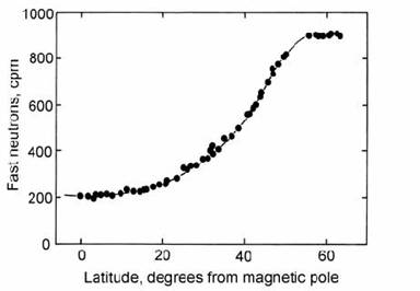
Fig. 14.1. Plot of cosmogenic neutron flux as a function of latitude to show the geographical variation in cosmic-ray-intensity. After Simpson (1951).
More recent evidence for the rate of atmospheric 14C homogenization came from atmospheric nuclear explosions. Fig. 14.2 shows the level of 14C at different locations around the world after the addition of excess 14C from atmospheric tests (Libby, 1970). Worldwide atmospheric homogenization occurs after only two or three years. The recovery rate of the Mojave Desert samples after 1965 suggests that the timescale for buffering of the atmosphere by surface ocean water is somewhat longer (17 years), but this is still very short relative to the 14C half-life.
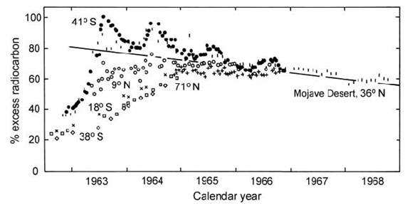
Fig. 14.2. Excess (bomb-produced) atmospheric 14C measured at different localities on the globe, during and after the peak of atmospheric nuclear testing. Localities: ( Q ) 71 oN; ( | ) the Mojave Desert, 36 oN; ( o ) 9 oN; ( H ) 18 oS; ( + ) 21 oS; ( <> ) 38 oS; ( ! ) 41 oS. After Libby (1970).
Libby (1952) also assumed that the atmosphere had a constant 14C activity through time, as a result of equilibrium between a constant rate of production and decay. Hence, the 14C activity of recent organic tissue was taken to be equal to the ‘initial’ activity of carbon samples formed in the past. A closed-system assumption was also argued on the basis that complex organic molecules cannot exchange carbon with the environment after death. (However, such exchange can occur in many carbonates, making them less reliable as dating material). The above-mentioned assumptions were supported (Arnold and Libby, 1949) by a good concordance between 14C dates and historical ages for a suite of test samples (Fig. 14.3). These ages were based on a 14C half-life of 5568 ” 30 yr obtained from a weighted mean of the four most precise laboratory counting determinations, all of which clustered closely around the mean.
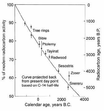
Fig. 14.3. Plot of measured 14C activity (disintegrations per minute per gram of carbon) in archaeological samples of known age against predicted activity based on modern wood and a 5568 yr half-life. After Libby (1952).
In the natural reduction of CO2 to carbon by photosynthesis and during laboratory preparation for analysis (e.g., combustion of carbon to CO2), isotopic fractionation between carbon isotopes can occur. This is due to the weaker bonding, and hence greater reactivity, of the lighter isotope (section 2.2.2). In order to assess the fractionation between 14C and 12C in natural and laboratory processes, Craig (1954) proposed that the 13C/12C ratio of samples be measured by mass spectrometry. Because fractionation is mass-dependent, 14C/12C fractionation will be twice as great as 13C/12C fractionation. The latter is normally expressed relative to the PeeDee belemnite (PDB) standard (Craig, 1957):
| (13C/12C)sample |
*13C = | )))))))) ! 1 | @ 103 [14.2]
| (13C/12C)PDB |
This fractionation factor can be directly converted into a correction to the 14C age using Fig. 14.4 (Mook and Streurman, 1983). In this diagram, normal * 13C compositions for various types of sample are shown. Because ‘modern wood’ is established as the reference point for calibrating the efficiency of 14C counting equipment, age corrections must be applied relative to this type of material (Fig. 14.4), which has a normal or ‘calibration’ value of *13C = !25 per mil (relative to PDB). In marine carbonates, this effect is offset by the 400 yr 14C age of ocean surface water, which must be subtracted from measured ages (section 14.1.6).
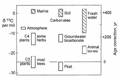
Fig. 14.4. Carbon isotope fractionation effects in different materials and necessary corrections to calibrated 14C ages for C3 plants (wood). Carbonates are hatched. After Mook and Streurman (1983).
14.1.1 14C measurement by counting
The development of the radiocarbon method went hand in hand with the development of low-level counting techniques. The specific activity of 14C is small, yielding a maximum count-rate of 13.6 decays per minute per gram (dpm/g) for modern wood, but only 0.03 dpm/g for a sample 50 kyr old. Furthermore, the maximum $ energy is low (156 keV), so that in a solid source of non-zero thickness a significant fraction of particles would be absorbed by other carbon atoms in the sample.
Libby’s early determinations of 14C activity were on samples of solid carbon using a ‘screen wall’ Geiger counter. However, this method was soon replaced by the analysis of CO2 in a gas counter (de Vries and Barendsen, 1953). CO2 is very readily prepared, and in the gas counter, there is no risk of losing counts (due to absorption) before the $ particles reach the detector.
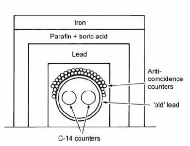
Fig. 14.5. Components in passive and active screening of a CO2 gas counter. After Mook and Streurman (1983).
Unfortunately the natural background level of activity which will be measured by a gas counter (cosmic rays and gamma emission from natural materials) is far larger than the level of activity from the sample itself. Hence, two screening techniques are used (Fig. 14.5). The first is a thick wall of material that itself has a low level of activity (e.g., ‘old’ lead). The second component is an array of Geiger tubes arranged immediately around the gas proportional counter. The Geiger tubes are electronically connected in anti-coincidence to the proportional counter. If a high-energy particle, such as a cosmic ray, enters the shielding, it will trigger the Geiger tubes at almost the same time as the proportional counter, and the two signals will cancel out. The dramatic effects of these shielding techniques on the counting background were demonstrated by Ralph (1971) using a counter filled with ‘dead’ CO2 made from anthracite coal.
Count rates (dpm) were:
No shielding: 1500
Shielded by iron and mercury: 400
Shielded and with anti-coincidence counters turned on: 8
Subsequent to Libby’s work, his dating assumptions and half-life value have been reexamined. However, it was decided to continue publishing radiocarbon ages using Libby’s atmospheric composition and half-life (Godwin, 1962). These are called ‘conventional ages’. Correction factors are subsequently applied to determine a true ‘historical’ age. We will now reexamine two of the most important assumptions.
14.1.2 Closed system assumption
Loss of carbon from a system during its geological lifetime is not usually a problem in radiocarbon dating. However, contamination with extraneous environmental carbon may be a major problem. To exclude such contamination, rigorous sample preparation procedures have been developed.
When dating wood or charcoal for archaeological purposes, the objective is to determine the time when the tree was cut down. Hence, it is only necessary to exclude post-mortem exchange with the environment.
For this, an Acid-Alkali-Acid leaching treatment, referred to as the AAA treatment, was found to be effective (Olsson, 1980). The three steps are:
1) Leach with 4% HCl at 80 oC for 24 hours to remove sugars, resins, soil carbonate and infiltrated humic acids.
2) Leach with up to 4% NaOH at up to 80 oC for at least 24 hours to remove infiltrated tannic acids (this step also removes part of the lignin).
3) Repeat step 1 to remove any atmospheric CO2 absorbed during the alkali step.
The overall process removes about 50% of the original carbon.
When dating tree rings for calibration studies (see below), the objective is quite different. In this case, it is essential to sample only material laid down in the year of growth corresponding to the annual ring. This requires that all material deposited during the subsequent life of the tree (e.g. lignin) must be leached away. This is accomplished by inserting a step 1a into the above procedure in which the wood chips are bleached by progressive addition of an almost equal weight of sodium perchlorate powder in dilute acetic acid at 70 oC. The procedure removes up to 75% of the carbon, leaving a residue of pure cellulose for analysis (Mook and Streurman, 1983).
When dating bones, all of the inorganic carbonate fraction must be removed by leaching with very dilute HCl because this fraction invariably exchanges carbon with groundwater. The organic carbon fraction in the bone is in the form of collagen, which is resistant to post-mortem exchange. Olsson et al. (1974) describes different methods for treating bones. Leaching with acid has also been shown to improve the accuracy of radiocarbon ages on corals (see below).
14.1.3 Initial ratio assumption
As radiocarbon measurements became more precise, systematic age discrepancies between historical material and radiocarbon dates began to suggest that the level of 14C activity in the atmosphere had varied with time. The first evidence for such temporal variations in 14C activity was provided by Suess (1955), who found that 20th-century wood showed a 2% depletion in activity relative to 19th-century wood. This was attributed to dilution of radioactive carbon by ‘dead’ carbon introduced into the atmosphere by burning fossil fuel (nuclear tests later drove the equilibrium in the other direction by adding 14C to the atmosphere). Subsequently, de Vries (1958) found that late-17th-century wood had ca. 2% higher activity than 19th-century wood. These two ‘anomalies’ are sometimes called the ‘Suess’ and ‘de Vries’ effects.
The discovery of secular variations in 14C activity has provoked various models that attempt to explain these variations. Forbush (1954) observed that the 11-year cycle of sunspot activity was inversely correlated with cosmic-ray intensity. This is because high levels of solar activity (marked by increased sunspot activity) cause an increase in the solar wind of ionised particles, which extends the Sun’s magnetic field and deflects galactic cosmic rays away from the Earth. Thus, calculations by Oeschger et al. (1970) suggest that the stratospheric cosmic-ray flux may be nearly doubled at solar minima, relative to maxima.
Because historical records are available for sunspot frequency, this provided a means of predicting past cosmic-ray intensity, and hence 14C production, over the last few hundred years. Stuiver (1961) performed these calculations and suggested that a sunspot minimum in the late-17th century could explain the ‘de Vries effect’ 14C activity maximum at that time. This was confirmed by Stuiver (1965) using more detailed 14C data (Fig. 14.6).
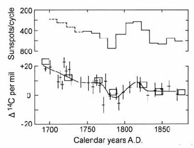
Fig. 14.6. Plots of sunspot activity and relative 14C activity, expressed as ), parts per mil, to show coherent anti-correlation in the 17th and 18th centuries. A best-fit curve is drawn using two 14C data sets (error boxes and error crosses). After Stuiver (1965).
Extension of the 14C activity curve to well before the time of Christ revealed large long-term variations, in addition to the short-term effects attributed to changes in solar cosmic-ray modulation (Suess, 1965). Elsasser et al. (1956) had predicted that if the strength of the Earth’s magnetic field displayed secular variations, as suggested by Thellier (1941 and following), then this would have affected the paleo cosmic-ray flux incident on the atmosphere, and hence 14C production.
However, strong evidence of a causal relationship with the Earth’s field strength was not established until Bucha and Neustupny (1967) provided more extensive paleomagnetic intensity measurements.
These data revealed sinusoidal variations in the Earth’s magnetic field strength which matched the sinusoidal deviations between radiocarbon and absolute ages.
By modeling the effect of paleomagnetic intensity variations on 14C activity, Bucha and Neustupny were able to match the deviations between tree-ring and radiocarbon time scales almost exactly (Fig. 14.7). A comparison with historically dated wood showed a very similar result, except that this curve was translated upwards by ca. 100 yr. This can be attributed to the average time delay between wood growth and utilization. Because the model of Bucha and Neustupny linked the long time-period deviations between radiocarbon and absolute ages to variations in the global magnetic field, it also implied that the deviations should be of a systematic worldwide nature. Hence, it gave grounds for the establishment of very precise calibration sequences, which could then be used for worldwide correction of ‘conventional’ radiocarbon ages to calendar ages.
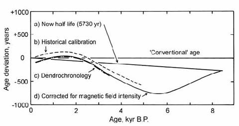
Fig. 14.7. Plot of age deviation between ‘conventional’ radiocarbon ages (half-life = 5568 yr) and other age determinations: a) radiocarbon method using 5730 yr half-life: b) historical time-scale; c) dendrochronology time-scale; d) using 5730 yr half-life and correction for variations in Earth’s magnetic field intensity. After Bucha and Neustupny (1967).
14.1.4 Dendrochronology
It was quickly realised that the most accurate way to calibrate the ‘conventional’ 14C time-scale for initial 14C variations was to integrate radiocarbon dates with tree-ring chronologies. Great efforts have been expended in this task over the last 30 years.
The longest dendrochronology calibration range has been achieved using the stunted bristlecone pine. When this work began the species was known as Pinus aristata. However, the great longevity of some populations of the bristlecone pine was subsequently recognized by placing these populations in a new species named Pinus longaeva. The semi-desert habitat of this tree gives rise to its great longevity and also permits good preservation of the dry wood after death. Thus, Ferguson (1970) erected a continuous master chronology reaching back over 7000 yr, based on several living trees and 17 specimens of dead wood from the White Mountains of eastern)central California (Fig. 14.8). This suite now extends nearly 8700 years (to 6700 B.C.), and includes the oldest living tree at more than 4600 years old! (Ferguson and Graybill, 1983).
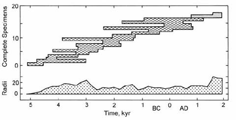
Fig. 14.8. A ‘master’ tree-ring chronology based on living and dead specimens of Bristlecone pine with overlapping age ranges. Upper chart shows range of each specimen. Lower chart shows total number of radii from which raw data were derived. After Ferguson (1970).
Suess (1970) presented a data set of 315 radiocarbon measurements for bristlecone pine from Ferguson’s collection, and used this data set to construct a continuous calibration curve from 5200 years B.C. to the present. One of the prominent features of this curve was the presence of numerous ‘wiggles’ with wavelengths of 100 ) 300 years, superimposed on the longer-term variations discussed above. Suess attracted much criticism because his calibration curve was drawn by eye through the measured points (with ‘cosmic schwung’), rather than using a statistical curve fit. Many other workers (as late as Pearson et al., 1977) maintained that the second order ‘wiggles’ identified by Suess were an artifact of statistical uncertainties in the data, and had no real meaning. However, this was illogical, since the known ‘de Vries effect’ wiggles of the 17th century A.D. were of similar magnitude. The reality of the ‘Suess’ wiggles in the ancient radiocarbon record (3500 years B.C.) was finally established by De Jong et al. (1979). These wiggles are seen superimposed on long-term 14C variations in the 9000 yr calibration curve shown in Fig. 14.9.
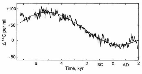
Fig. 14.9. Changes in atmospheric 14C activity in the last 9000 years, presented in the form of isotopic fractionation per mil, based on ‘continuous’ Bristlecone pine and ‘floating’ European oak chronologies. The apparent fit to a sinusoidal function is now known to be coincidental. After Bruns et al. (1983).
Comparatively large (20 per mil) 14C variations in wood from single sunspot cycles have been claimed by some workers (e.g. Baxter and Farmer, 1973; Fan et al., 1986). However, atmospheric 14C variations on this time-scale are not consistent with the experimental data of Stuiver and Quay (1981). The latter workers modelled small (4 per mil) 14C variations over sunspot cycles which are at the limits of measurement precision.
The convoluted shape of the calibration curve introduces ambiguities to 14C dating within many periods, since a single radiocarbon age can correspond to more than one historical age. These ambiguities may sometimes be resolved by applying historical constraints (e.g. section 14.2.1). Alternatively, they may be avoided in the dating of wood samples, if a piece spanning more than about 50 growth rings can be dated. This ring sequence then forms a small ‘floating’ calibration curve which can be ‘wiggle matched’ with the known calibration curve to yield a much more accurate time-span for the growth of the sample wood. Suess and Strahm (1970) demonstrated this technique when they dated a floating tree ring sequence from Auvernier (Switzerland) against the bristlecone pine calibration curve (Fig. 14.10). This procedure allowed the age uncertainties on the Auvernier material to be reduced from hundreds of years to decades.
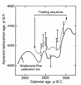
Fig. 14.10. Comparison of 14C data for a wood sample and the calibration curve to show the application of ‘wiggle matching’. The dashed line is the proposed fit to the measured data, shown with error bars. After Suess and Strahm (1970).
In order to obtain the highest quality calibration curve, it is desirable to analyse samples representing single annual rings. However, the small size of the bristlecone pine limits the precision which can be obtained, because of the limited amount of sample for analysis. Therefore, other work has been devoted to obtaining a more detailed calibration curve from larger trees (e.g. De Jong et al., 1979).
In Europe, the most important tree for detailed calibration purposes is the oak (Quercus petraea). This is partly because the oak very rarely has missing annual growth rings. In contrast, the widespread Alder may lack up to 45% of its annual rings (Huber, 1970). The oak is also ideal because it is a long-lived, large tree which displays good resistance to decay after death. In North America, the last 1500 yr of the 14C timescale has been calibrated in great detail (Stuiver and Pearson, 1986) using large trees such as the Douglas fir (Pseudotsuga menziesii) and Giant redwood (Sequoia gigantea). This curve was adopted as a new international standard at the 1985 Radiocarbon business meeting (Mook, 1986). Part of this curve is used below (section 14.2.1).
Even more exact dates are possible if the floating chronology comes from an area geographically near to the calibration chronology. Having ‘wiggle matched’ the radiocarbon data to obtain historical ages with uncertainties of a few decades, the widths of the tree rings themselves are then matched between the floating and calibration material, to obtain an exact date. However, this procedure is only possible if the two chronologies come from areas with the same weather pattern, thus giving rise to similar growth variations.
Hillam et al. (1990) used this procedure to date a Neolithic wooden walkway from Somerset (England) to the probable year of its construction (3806 B.C.). This age is based on the fact that ten timbers had bark surfaces with ages of 3807/3806 B.C., and must therefore have been cut down in that calendar year. A single sample with a bark age of 3800 B.C. probably represents a later repair to the walkway. This work suggests that as dendrochronologies are completed for more areas of the world, it should increasingly be possible to date large wood samples to the exact age of their felling.
In principle, it should also be possible to create a floating radiocarbon sequence by the analysis of several plant macro-fossils (such as seeds) from a soil sequence. Such a sequence could then be wiggle-matched to the dendro-calibration to determine a more much reliable calendar age than is possible from the calibration of single radiocarbon ages.
14.1.5 Production and Climatic effects
Many attempts have been made to extend the calibrated radiocarbon time-scale beyond the limit of dendrochronology. Early work was mainly based on varved lake sediments (e.g. Tauber, 1970) or ice cores (e.g. Hammer et al., 1986). Sediment varves are usually caused by a change in the type of minerals being deposited at different times of the year, but are not as reproducible as tree rings. For example, if sediment from the bottom is stirred up by strong winds and then redeposited, it may be possible for more than one varve layer to be deposited in a year. As a result, many different and conflicting calibration lines were proposed, which largely discredited this approach.
Bard et al. (1990a) took a major step forward in extending the radiocarbon calibration using mass spectrometric U)series analysis (section 12.2.1). This method was used to assign absolute ages to Barbados corals previously analysed for 14C. In view of uncertainties about closed system behaviour in carbonates, the method was tested by analysis of samples less than 10 kyr old. These gave ages in good agreement with the dendrochronology timescale, after applying a 400 yr correction for 14C equilibration between atmospheric and surface seawater (the ‘reservoir age’).
Results for older samples were presented on a plot of )14C activity (relative to modern wood) against U)Th age (Fig. 14.11). Samples in the range 10 ) 15 kyr gave )14C activities well within error of those predicted from geomagnetic field strength data. Samples older than 15 kyr initially gave more scattered data. However, repeat analysis of the 14C measurements after strong acid leaching gave more consistent results (Bard et al. 1993, 1998).
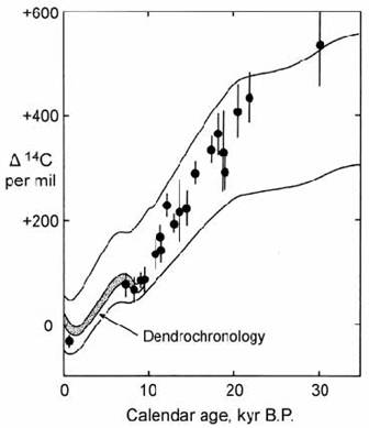
Fig. 14.11. Plot of )14C activity in corals (relative to modern wood) against U)Th ages. Heavy curve = dendrochronological calibration. Dashed lines show the envelope of 14C activity predicted from a theoretical cosmogenic model. After Bard et al. (1993).
Because the atmosphere contains only 5% of the carbon budget of the ocean)atmosphere system, climatic changes might have had a major influence on atmospheric 14C abundances, modifying the effects of cosmogenic radiocarbon production. Large effects are not expected during the Holocene period covered by the dendrochronological timescale due to its relatively consistent climate. However, much larger climatic effects are expected during the last glacial cycle. Therefore, the use of U-series dating to extend the calibrated timescale further back in time allows a test to be made of these effects on atmospheric 14C abundances.
Mazaud et al. (1991) compared the coral data of Bard et al. (1990a,b) with a 14C production model based on an improved geomagnetic intensity record. The good agreement between the coral data and the predicted 14C activity curve means that long-term activity variations in the atmosphere and hydrosphere can be largely explained by variable cosmogenic production (in response to secular variations in the magnetic field). Hence, climatic effects, which can affect the 14C equilibrium between atmospheric and marine carbonate reservoirs, must play a subordinate role. However, Stuiver et al. (1991) argued that climate could have a second-order effect on atmospheric 14C/12C activity ratios by releasing 12C from oceanic carbonate sinks through changes in ocean circulation.
A continuous record of atmospheric radiocarbon through the period of the last glacial cycle was obtained by Beck et al. (2001) from a cave stalagmite, precisely dated by U-series analysis. The stalagmite records atmospheric radiocarbon signatures through the medium of dead plant material in soils, which provides the majority of dissolved carbon in cave groundwater. However, it was necessary to correct for contamination by a subordinate amount of dead radiocarbon leached from the limestone wall rocks of the cave. Nevertheless, comparison with coral, varve, and dendrochronologies over ranges of several thousand years showed relatively constant offsets, which could then be corrected. The results in the period from 30 to 45 kyr ago showed very dramatic variations of ) 14C. These results were broadly consistent with evidence for enhanced cosmogenic nuclide production during this period from 10Be evidence (section 14.3.4). However, variation of climatic parameters (in addition to geomagnetic variation) was necessary to explain the full magnitude of the enhanced atmospheric 14C abundance peak between 30 and 40 kyr BP.
The most recent climatic event which may have caused a perturbation in the ocean–atmosphere carbon balance is the Younger Dryas event, a brief glacial re-advance that occurred between 13 and 11.5 kyr BP. Hence, this event has proved to be a testing ground of high-precision 14C measurements designed to compare atmospheric 14C abundances with production rates. The first of these detailed studies was made by Edwards et al. (1993a) using a coral record from 8 ) 14 kyr B.P. They found a markedly rapid decrease in 14C activity between 12 and 11 kyr B.P., which they attributed to dilution of atmospheric 14C by ‘dead’ carbon as a result of the Younger Dryas event. Hence, it was argued that climatic changes could perturb the overall control of the geomagnetic field on atmospheric 14C activity for short periods of time.
Further investigation of this problem was made using two new varved sediment records. The first example is from Lake Suigetsu, near the coast of Central Japan (Kitagawa and van der Plicht, 1998). This small freshwater lake has a water depth of 34 m, but contains a 75 m-deep thickness of sediment at its bottom. The sediment shows annual varves about 1 mm thick, formed by variation from a winter season of dark clay deposition to a spring season of white (siliceous) diatom deposition. The sediments were cored, and the most clearly banded section from 10 m to 30 m depth showed 29,100 varves. From within this section, 250 samples of wind-blown plant debris and insect wings were dated by radiocarbon, allowing this section to be anchored to the tree ring calibration curve between 9000 and 11,000 years BP.
The second new calibrated varve section was formed by marine sediments in the (marine) Cariaco Basin of the Caribbean (Hughen et al., 1998). The dated points in this sediment core showed exceptionally good agreement with the tree ring calibration curve and with dated coral samples in the range from 9000 to 12,000 years BP (Fig. 14.12). Unfortunately there was some minor disagreement with U)Th dated coral determinations around 13,000 years BP. However, the Cariaco basin results agree with Lake Suigetsu in predicting a sharp spike in ) 14C at this time.
These data were compared with new predictions of atmospheric radiocarbon production during the Younger Dryas by Muscheler et al. (2000). This prediction was obtained from a record of 10Be production from the GISP2 ice core in central Greenland (section 14.3.3) using a box model for radiocarbon exchange between the atmosphere and oceans. The results were in good agreement with predicted variations in ) 14C back to 12 kyr BP, but failed to fully explain the magnitude of the observed radiocarbon spike at the Younger Dryas (Fig. 14.12). Hence, Muscheler suggested that additional climatic effects were needed to explain the Younger Dryas peak, possibly involving changes in ocean circulation.
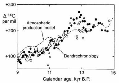
Fig. 14.12. Radiocarbon measurements for the Cariaco basin varve section ( ! ), showing excellent agreement with the dendrochronology calibration line (shaded band) and U)Th dates on corals ( ” ). Dotted line = production model. After Marchal et al. (2001).
The opposite case was argued by Goslar et al. (2000) on the basis of varve records from Polish lakes. The radiocarbon data from these lakes are more scattered than the two examples cited above. However, a large clump of data was found in the time interval between 13,000 and 12,500 years PB which lay below the varve record in Fig. 14.12, but in agreement with U–Th coral data (open symbols in Fig. 14.12). On this basis, Goslar et al. argued that the model of radiocarbon production based on the 10Be ice core record was capable of explaining most of the observed radiocarbon variation and, therefore that it was not necessary to invoke changes in ocean–atmosphere 14C partition due to ocean circulation. Further modelling by Marchal et al. (2001) supported the arguments of Muscheler et al. (2000), but it was admitted that a decisive conclusion was not yet possible.
14.1.6 Radiocarbon in the oceans
Radiocarbon is a very useful tracer in oceanography because it allows quantitative estimates to be made on the residence times of water at different depths, the mixing between different water bodies, and the magnitude of ocean currents. Radiocarbon evolution in the oceans begins with ‘ventilation’ of surface water to the atmosphere, which allows this water to reach equilibrium with atmospheric radiocarbon. After a water body moves away from the surface, it can be dated by the decay of this radiocarbon, and hence its flow path and mixing history can be traced.
Studies of the radiocarbon budget of the oceans began in the 1950s at the same time as the first atmospheric nuclear tests, which produced large quantities of C-14 by neutron activation of nitrogen. This ‘bomb’ radiocarbon complicates the interpretation of natural radiocarbon variations in the oceans, but the entry of this ‘spike’ of anthropogenic radiocarbon into the oceans also provides a useful tracer of the very recent movement of water bodies. However, because the radiocarbon method was in its infancy when atmospheric nuclear testing began, there was an inadequate data set of pre-bomb measurements on seawater to provide a proper baseline to evaluate the magnitude of the bomb signature. Hence, a full understanding of the early data sets was not achieved until later studies revealed the composition of pre-bomb radiocarbon inventories. For example, the analysis of corals provides a means of sampling pre-bomb radiocarbon signatures of the surface oceans (Druffel, 1996).
The first major program for the radiocarbon analysis of ocean water, called GEOSECS (Geochemical Ocean Sections Study) was undertaken in the mid 1970s, near the peak of bomb radiocarbon in the atmosphere. Hence, surface water analyses from this program provide a dramatic picture of the effects of ocean currents on the bomb radiocarbon signature (Fig. 14.13). The highest values of bomb radiocarbon were found in the sub-tropics, where water has the longest surface residence time. In contrast, Antarctic water was found to have essentially no bomb radiocarbon signature, which was attributed to strong mixing between surface water and deep water (e.g. Nydal, 2000). Comparison of radiocarbon data from the GEOSECS program with more resent sampling programs such as WOCE (in the early 1990s) showed a diminution with time of the bomb signature in the surface ocean (Fig. 14.13), but also revealed a concomitant increase of the bomb signature in the deep ocean (e.g. Ostlund and Rooth, 1990).
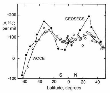
Fig. 14.13. Radiocarbon variations in surface ocean waters of the Pacific as a function of latitude, attributed to atmospheric nuclear tests. ( ! ) = GEOSECS; ( ” ) = WOCE. After Key et al. (1996).
Natural radiocarbon variations in the oceans provide evidence about ocean circulation on a longer time scale. The first detailed radiocarbon study of the Atlantic Ocean was made by Broecker et al. (1960). After correction for anthropogenic contamination, tropical waters were found to have a ) 14C composition of –50 per mil (relative to 19th century wood), equivalent to an apparent 14C age of ca. 400 yr. As they flow north, these waters impart the same apparent 14C age to North Atlantic surface water. After mixing with cold Arctic water, they feed North Atlantic Deep Water (NADW) with ) 14C values beginning around –70 parts per mil. However, as this deep water moves southward, 14C activities fall progressively as the water body ages, reaching a ) value of –160 in Antarctic bottom water.
These results are consistent with the established oceanographic model for the Atlantic (Fig. 4.37). In this model, tropical waters are transported (advected) to the North Atlantic, where they cool and, because of their high salinity, sink to form North Atlantic Deep Water (NADW). This body of deep salty water flows southward to the Antarctic and, after mixing with Antarctic bottom water, ultimately reaches the Pacific. The role of the Antarctic Ocean as a mixing zone between young Atlantic water (NADW) and older deep water from the Pacific and Indian oceans was confirmed by a large radiocarbon data set from the GEOSECS program (Stuiver et al., 1983), as shown in Fig. 14.14.
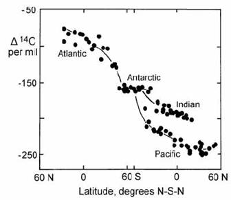
Fig. 14.14. Plot of ) 14C against latitude, showing the progressive drop in radiocarbon activity from the North Atlantic, through the Antarctic mixing zone, to the Pacific/Indian oceans. After Stuiver et al. (1983).
If the change in ) 14C from North Atlantic surface water to Pacific Deep Water was due entirely to radiocarbon decay (at ca. 11 per mil / century), this would imply a total age of ca. 1700 yr since the time when this water was last at the sea surface. However, the ‘true’ age of a water body, defined as the average time since the water in that package was at the sea surface, is considerably less. This is demonstrated by the use of a General Circulation Model (Campin et al., 1999). The results of this modelling for the present day Atlantic Ocean are shown in Fig. 14.15. At the top, Fig. 14.15a shows that the model successfully recreates the radiocarbon age structure of NADW and the old radiocarbon age of Antarctic Bottom Water (AABW). However, Fig. 14.15b shows that the true age of AABW is much lower. The difference is due to the presence of sea ice, which prevents the ventilation of radiocarbon from Antarctic surface water to the atmosphere. Furthermore, the average mixing time in each individual ocean basin is much shorter than the radiocarbon age: ca. 200–300 yr in the Atlantic, 500 yr in the Pacific, and only 80 yr in the Antarctic.
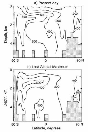
Fig. 14.15. Predicted ages of Atlantic water (contoured) based on a general circulation model for the oceans. a) apparent radiocarbon age (above the surface water value of 360 yr); b) actual water age since surface residence. After Campin et al. (1999).
14.1.7 The ‘Ocean Conveyer Belt’
The global system of deep water transport from the North Atlantic, via the Antarctic, to the Pacific has been termed the oceanic Thermo-Haline Circulation (THC) or the Ocean Conveyer Belt (Broecker and Denton, 1989). These authors suggested that this thermohaline circulation (Fig. 14.16) played a critical role in controlling climate switches between glacial and interglacial periods. For example, evidence from elemental tracers suggested that the conveyer belt might have been ‘turned off’ during glacial periods, which would have tended to amplify the cooling effect in the North Atlantic by preventing the export of cold NADW and the import of warm tropical water. Broecker and Denton also speculated that a similar effect occurred during the Younger Dryas event, the temporary glacial re-advance which interrupted the last deglaciation.
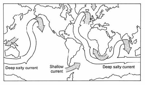
Fig. 14.16. World map showing the deep water ‘ocean conveyer belt’ connecting major world oceans. Shaded arrows = surface water currents. After Broecker and Denton (1989).
Radiocarbon analysis of biogenic carbonates of different ages can be used to study changes in the operation of the Ocean Conveyer Belt by comparing the apparent ages of a given water mass at different times. For example, comparison between the radiocarbon ages of benthic and planktonic forams in a given deposit allows the relative radiocarbon ages of local surface and deep water bodies to be compared. This work was not possible until the advent of Accelerator Mass Spectrometry (see below) because of the small amount of sample material available. The first study was attempted by Andree et al. (1985) but was complicated by the effects of bioturbation because the core under study had a sedimentation rate of only 1.5 cm/kyr.
Shackleton et al. (1988) avoided these problems by working on a core from the Central Pacific with a sedimentation rate of 10 cm/yr. For each sampled increment of the core (typically 2 ) 3 cm) the difference between the radiocarbon ages of benthic and planktonic forams gave a ‘ventilation age’ for Pacific Deep Water, representing the time since this water body equilibrated with the atmosphere at the sea surface. These values were plotted against the radiocarbon age of surface water, determined by subtracting a ‘reservoir age’ of 650 yr (representing the apparent radiocarbon age of Pacific surface water) from the ‘conventional age’ determined analytically. The data are compared in Fig. 14.7 with the 1500 yr ventilation age of present day Pacific Deep Water, measured in the GEOSECS program. The results of Andree et al. (1985) are also shown for comparison. The ventilation ages measured by Shackleton et al. were quite variable, especially during the period of deglaciation 18 ) 12 kyr BP. However, they argued that it was possible to identify a ‘glacial mean value’ that was about 500 years older than the ventilation age of Pacific Deep Water at the present day. Subsequent work has also reported considerable scatter in ages, but has generally agreed with this conclusion.
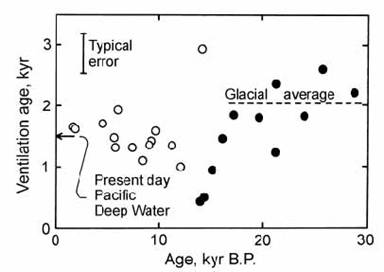
Fig. 14.17. Plot of apparent ‘ventilation’ age for Pacific Deep Water based on differences in radiocarbon ages between planktonic and benthic forams from a Central Pacific core. ( ” ) = data of Andree et al. (1986). ( ! ) = new data, after Shackleton et al., (1988).
While B)P (benthic)pelagic) ages give a reasonable approximation to the ventilation age of ocean water masses, Adkins and Boyle (1997) pointed out that there were inaccuracies in this method, particularly when atmospheric radiocarbon abundances were changing rapidly in response to changing cosmogenic production. For example, during a period of decreasing atmospheric 14C abundances (as seen for much of the past 20 kyr), the initial radiocarbon activity of an old deep-water sample would have been higher (when that water body was at the sea surface) than the activity level in surface water by the end of the period of evolution of the deep water body. This causes B)P ages to under-estimate the true ventilation age of the water body.
To avoid this inaccuracy, Adkins and Boyle proposed an improved calculation method which they termed the ‘projection’ age method. This involves projecting the evolution line of the deep water sample back in time until it reaches the atmospheric evolution curve (Fig. 14.18). The ventilation age is then calculated by subtracting the ‘reservoir age’ of surface ocean water. The method is based on the premise that the principal cause of changes in atmospheric 14C abundance is production variation, rather than changes in ventilation (since the latter would create a circular argument). In addition, it must be assumed that mixing of waters has not occurred. The result of applying this method to previously determined ventilation ages was to slightly increase the average ventilation age for Pacific Deep Water during the last glacial maximum to a value of 600 years above the present day value.
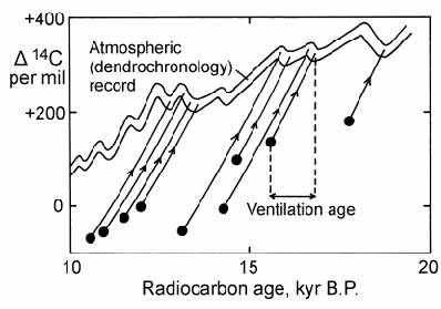
Fig. 14.18. Plot of ) 14C against time to illustrate the ‘projection method’ for calculating ventilation ages of deep water bodies relative to atmospheric radiocarbon. After Adkins and Boyle (1997).
Another consequence of a slow-down in the ocean conveyer belt would be a reduction in the northward flow of tropical water to the North Atlantic, causing the apparent ‘equilibration age’ of North Atlantic surface water to rise. Bard et al. (1994) attempted to test this prediction for the Younger Dryas period by comparing the 14C ages of plant fossils and planktonic forams of this age, marked by the distinctive Vede ash bed. The difference between terrestrial and planktonic radiocarbon ages would yield the equilibration age for North Atlantic surface water during the Younger Dryas period.
Data from four North Atlantic cores gave an average 14C age 1400 yr older than the terrestrial section. However, because the ‘control’ samples of plant material used to determine atmospheric radiocarbon abundance did not come from the same cores as the forams, a 650 yr correction was necessary to account for marine bioturbation of the foram samples (despite the relatively high sedimentation rate in the core). This left a net age difference of about 750 yr, representing the estimated ‘reservoir age’ during the Younger Dryas. It compares with a present day reservoir age of 400 yr for the North Atlantic, as described above. The increased North Atlantic reservoir age during the Younger Dryas was attributed by Bard et al. to reduced ventilation of North Atlantic surface water to the atmosphere. Some of this difference could be accounted for by increased sea ice cover during the Younger Dryas, but the preferred model of Bard et al. was a reduction in the formation of NADW.
Deep-sea corals represent an alternative source of information about the radiocarbon signatures of deep water masses. These corals are slow-growing solitary corals that do not rely on symbiotic algae for an energy source, and can therefore grow outside the range of reef-building corals, in the deep sea and in polar regions. These corals can offer high-resolution climatic records because, unlike deep-sea sediments, they are not affected by bioturbation. As with the B–P method, ventilation ages from deep-sea coral analysis have been somewhat scattered (e.g. Goldstein et al., 2001). However, this may partly reflect the variable ‘residence’ ages of surface water, which must be subtracted from the apparent radiocarbon ages of deep water corals in order to calculate the ventilation age. For example, ventilation ages of very young deep-sea corals from the South Pacific gave results that were sometimes in agreement with the corresponding water masses, and sometimes not (Fig. 14.19). Agreement between coral and GEOSECS data was very good for the sample from 950 m depth, but less good for samples from 100 m and 350 m depth. However, Goldstein et al. suggested that part of the miss-fit for the shallowest point may be due to contamination of the coral sample by bomb radiocarbon in the water mass in which it grew.
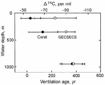
Fig. 14.19. Plot of ventilation age against depth for the south Pacific, to compare ages for deep-sea corals ( ! ) with GEOSECS data on seawater ( ” ). After Goldstein et al. (2001).
Because of these problems, it is likely that ventilation ages from both corals and forams are subject to considerable sampling ‘noise’. However, averaging from several different sampling sites can help to overcome this noise. Based on such a approach, Goldstein et al. (2001) determined that glacial bottom water from the Last Glacial Maximum (LGM) had an average ventilation age 1360 yr older than present day bottom waters sampled in the GEOSECS program. This supports the proposal of Broecker and Denton (1989) that the Ocean Conveyer Belt operated at a slower pace during glacial periods.
REFERENCES
Adkins, J. F. and Boyle, E. A. (1997). Changing atmospheric ) 14C and the record of deep water paleoventilation ages. Paleoceanography 12, 337–44.
Anderson, E. C. and Libby, W. F. (1951). World-wide distribution of natural radiocarbon. Phys. Rev. 81, 64)9.
Andree, M., Oeschger, H., Broecker, W., Beaven, N., Klas, M., Bonani, G., Hoffman, H. J., Suter, M., Woelfli, W. and Peng, T.-H. (1986). Limits on ventilation rates for the deep ocean over the last 12,000 years. Climate Dynamics 1, 53–62.
Andrews, J. N., Davis, S. N., Fabryka-Martin, J., Fontes, J. C., Lehmann, B. E., Loosli, H. H., Michelot, J-L., Moser, H., Smith, B. and Wolf, M. (1989). The in situ production of radioisotopes in rock matrices with particular reference to the Stripa granite. Geochim. Cosmochim. Acta 53, 1803)15.
Arnold, J. R. (1956). Beryllium-10 produced by cosmic rays. Science 124, 584)5.
Arnold, J. R. (1958). Trace elements and transport rates in the ocean. 2nd UN Conf. on Peaceful Uses of Atomic Energy 18, 344)6. IAEA.
Arnold, J. R. and Libby, W. F. (1949). Age determinations by radiocarbon content: Checks with samples of known age. Science 110, 678)80.
Bard, E., Arnold, M., Fairbanks, R. G. and Hamelin, B. (1993). 230Th)234U and 14C ages obtained by mass spectrometry on corals. Radiocarbon 35, 191)9.
Bard, E., Arnold, M., Hamelin, B., Tisnerat-Laborde, N. and Cabioch, G. (1998). Radiocarbon calibration by means of mass spectrometric 230Th/234U and 14C ages of corals: an updated database including samples from Barbados, Mururoa and Tahiti. Radiocarbon 40, 1085–92.
Bard, E., Arnold, M., Mangerud, J., Paterne, M., Labeyrie, L., Duprat, J., Melieres, M. A., Sonstegaard, E. and Duplessy, J. C. (1994). The North Atlantic atmosphere–sea surface 14C gradient during the Younger Dryas climatic event. Earth Planet. Sci. Lett. 126, 275–87.
Bard, E., Hamelin, B., Fairbanks, R. G. and Zindler, A. (1990a). Calibration of the 14C timescale over the past 30,000 years using mass spectrometric U)Th ages from Barbados corals. Nature 345, 405)10.