
Cosmic rays interact directly with nitrogen and oxygen atoms in the atmosphere, causing spallation (fragmentation) into the light atoms Li, Be, and B. Amongst these, one of the nuclides produced is the unstable isotope 10Be. Cosmogenic 10Be can also be generated in the surface layer of exposed rocks by in situ production. However, this subject will be dealt with in a later section.
10Be decays by pure $ emission to 10B. It was first observed in naturally occurring material by radioactive counting (Arnold, 1956). However, even at that time, Arnold recognized that mass spectrometry might supplant radioactive counting as a method for the determination of 10Be. This is because the relatively long half-life of 1.51 Myr (Hofmann et al., 1987) makes counting a very inefficient process for 10Be analysis of natural samples. For example, McCorkell et al. (1967) used 1200 tonnes of ice-water to make 10Be (and 26Al) measurements by $ counting on Greenland ice. In contrast, Raisbeck et al. (1978) made the first AMS measurement on similar material using only 10 kg of ice water.
Analytically, 10Be determination by AMS is similar to 14C, but involves some additional complications. Because Be does not form stable negative ions, the BeO! species must be used, upon which the isobaric interference of 10BO is a serious problem. This is overcome by passing the ion beam through an absorber gas (in front of the detector) whose pressure is adjusted to completely stop 10B transmission. The high ion velocity of the 10Be beam generated by AMS allows this species to pass through to the detector, which consists of a gas ionisation counter in front of a surface barrier detector which finally absorbs the ion beam. The first detector measures energy loss () E) of the ions as they collide with gas molecules in the chamber (this property of the ions is inversely proportional to their atomic number). The second detector measures residual energy. Using this bivariate discriminant, 10Be ions can be resolved from all other signals (Fig. 14.23) to yield a very low background. 10Be contents of samples are measured relative to added 9Be spike, and normalised for machine mass discrimination by frequent standard analysis.
Related Articles:
All About Cosmogenic Nuclides – Part One
What is Accelerator Mass Spectrometry
Fig. 14.23. Plot of )E against E for a typical geological sample, to show resolution of 10Be from other species. Dot size indicates the number of counts in each bin (smallest = 1 count). After Brown et al. (1982).
14.3.1 10Be in the atmosphere
10Be enters the hydrological cycle by attachment to aerosols, from which it is scavenged by precipitation. Consequently, it has a very short (ca. 1 week to 2 yr) residence time in the atmosphere and, unlike 14C, is not homogenized within the atmosphere prior to its fallout.
It was originally intended (Raisbeck et al., 1979) that 10Be analysis of rainwater would allow accurate constraints to be placed on the global average 10Be production rate. However, two factors complicate the determination of the 10Be flux in rainwater. One is the tendency for comparatively Be-rich soil particulates to be caught up in the atmosphere and cause secondary contamination of rain (Stensland et al., 1983). Once this effect is removed, individual depositional events still turn out to have very variable 10Be contents (Brown et al., 1989).
One way of gauging the effect of soil re-suspension on 10Be abundances is to compare them with 7Be data. The latter species has relatively similar atmospheric production rates to 10Be, but much lower levels in soils due to its very short (53 day) half-life. It is measured by ( counting. An alternative way of assessing the effects of soil re-suspension is to compare continental and oceanic 10Be deposition rates. Brown et al. (1989) used both of these approaches in an analysis of 10Be precipitation in Hawaii and the continental US to test its behaviour at temperate latitudes. Average 10Be contents of Hawaiian rain, in which atmospheric soil suspension is negligible, are very similar to 7Be in rain from Illinois in the US (Fig. 14.24), but in both cases a few events yield very large relative contents.
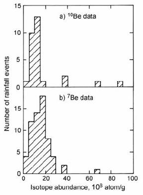
Fig. 14.24. Histograms of 10Be and 7Be concentration respectively in rainfall from Mauna Loa, Hawaii and Bondville, Illinois. The former are weekly rainfall aggregates, the latter represent individual showers. After Brown et al. (1989).
The variability of 10Be contents in individual rain showers makes it difficult to determine accurate annual fluxes for mid-latitudes. A summary of these data as a function of latitude (Fig. 14.25) shows the variability of these estimates (Brown et al., 1992). However, at tropical latitudes the estimates of annual 10Be flux are more reproducible. The latter are in good agreement with a global 10Be flux estimate of 106 atom/cm2/yr, based on cosmic-ray intensity as a function of latitude (Lal and Peters, 1967). Therefore, at the present time, the curve in Fig. 14.25 represents the best available estimate of the atmospheric 10Be flux.
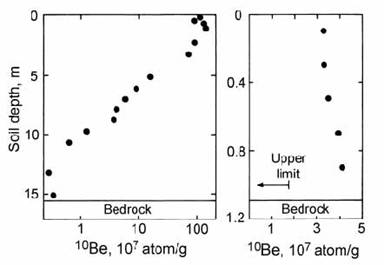
Fig. 14.25. Summary of empirical estimates of annual 10Be flux in rainfall, as a function of latitude. These are compared with a theoretical production curve based on cosmic-ray intensity. After Brown et al. (1992).
14.3.2 10Be in soil profiles
Beryllium is partitioned very strongly from rain water onto the surface of soil particles such as clay minerals. If we assume that 10Be adsorption is perfect, and that a given soil section is developed by weathering of rock or rock debris without the addition or removal of sediment during the weathering process, the soil section should contain a complete inventory of all deposited 10Be that has not yet decayed. This process offers the opportunity of dating a soil profile by measuring the total accumulation of 10Be in the section, but it is apparent that there are a large number of assumptions.
The 10Be inventory of a soil profile in Virginia represents a case where beryllium uptake appears to be nearly 100% efficient (Pavich et al., 1985). 10Be activities display a smooth decay curve against depth (Fig. 14.26a), with a total inventory of 9 H 1011 atom/cm2. We can compare this value with a theoretical inventory, N, assuming 100% uptake over a given period of time. This is given by the equation:
q
N = ) (1 ! e!8 t) [14.3]
8
where q is the input flux from rainfall and t is the accumulation time. If the profile is infinitely old, relative to the 1.5 Myr half-life of 10Be, it will reach saturation, whereupon input flux from rainfall is balanced by the rate of decay (8). Equation [14.3] then simplifies to N = q/8. Given an annual deposition flux of 1.3 H 106 atom/cm2 at this latitude, the saturation inventory will be 3 H 1012 atom/cm2, which is three times the observed inventory. The discrepancy can be explained by loss of 10Be-enriched soil from the top of the profile by erosion, and its replacement at the bottom of the profile by weathering of bedrock with no 10Be. Solving equation [14.3] for t (using the observed inventory) yields the residence time of 10Be in the profile, equal to 800 kyr.
Very different 10Be behaviour is demonstrated by a soil profile from the Orinoco Basin (Fig. 14.26b), which has a total inventory of only 5 H 109 atom/cm2. Assuming an annual 10Be flux for this latitude of 0.4 H 106 atom/cm2, we obtain a 10Be residence period in the soil profile of only 12 kyr (because t is short relative to the 10Be half-life, it can be approximated by N/q). This low value is best explained by ‘breakthrough’ of 10Be from the base of the profile by leaching (Brown et al., 1992).

Fig. 14.26. Plots of 10Be activity as a function of depth in two soil profiles. a) Virginia Piedmont, after Pavich et al. (1985); b) Orinoco Basin, after Brown et al. (1992).
Differences in 10Be retention between the two cases described above can be understood in the light of laboratory experiments on beryllium partition between soil and water (You et al., 1989). These studies showed that beryllium retention on soil particles is strongly pH-dependent, with distribution coefficients of ca. 105 in neutral conditions (pH 7) but less than 100 at pH 2. Hence, the more acidic conditions in tropical soils are less favourable for beryllium retention.
In alkaline soils, beryllium mobility within the soil profile may be very limited, and in these conditions, 10Be may be used as a stratigraphic tool. An example is provided by a 10Be study of Chinese loess, in which carbonate-rich conditions yield a pH value of 8 (Chengde et al., 1992). The profile was dated magnetically back to 800 kyr, and represents the products of wind-borne deposition through varying climatic conditions. Chengde et al. tuned their profile to the Quaternary climatic record provided by sea-floor 18O variations. They concluded that during arid periods, rapid loess deposition was accompanied by high fluxes of 10Be, adsorbed onto wind-blown particles. These sections were interspersed with wetter periods with lower 10Be depositional fluxes.
14.3.3 10Be in snow and ice
Atmospheric 10Be accumulates in snow and ice, but its half-life is too long to date such deposits. However, it can be used as a tracer of climatic changes and to understand the processes modulating cosmogenic 14C production in the atmosphere. The first detailed study of this type was made by Raisbeck et al. (1981a) on a 906 m-long ice core from the Dome C station, eastern Antarctica. This core had been dated on the basis of oxygen isotope correlations with 14C-dated marine sediments. A detailed analysis of the top 40 m of core revealed a 10Be maximum around 1700 A.D., which correlated with the 14C de Vries effect maximum (section 14.1.3) and the ‘Maunder’ sunspot minimum at this time (Eddy, 1976). Consequently, these data supported the solar modulation of cosmic-ray intensity model.
Subsequent studies of Greenland ice cores from the Camp Century and Milcent stations (Beer et al., 1984) confirmed the 10Be maximum associated with the Maunder sunspot minimum. In addition, Beer et al. (1985) performed a Fourier transform analysis of very detailed isotopic data from the Milcent core. This revealed second order 10Be variations with a 9 ) 11 year cycle time equal to the ‘sunspot cycle’, both before and during the Maunder minimum. Hence, Beer et al. concluded that solar activity continues to vary, even when sunspots are not actually visible.
Studies of the solar modulation of 10Be production were extended to a 1000 year period in a more recent study from the South Pole (Bard et al., 1997). This section was precisely dated using 20 impurity layers which were correlated with known volcanic eruptions. In this section, the peak at the Maunder Minimum (1700 AD) is seen very sharply, but similar peaks are also visible at other periods, particularly around 1050 AD (Fig. 14.27). Measurement of 10Be in polar ice is particularly effective to study solar modulation of cosmogenic production because the shielding effect of the Earth’s magnetic field is reduced at the poles, enhancing the sensitivity of cosmogenic production to the effects of the solar wind. Furthermore, these local production effects are fully transmitted into the ice core record because 10Be is not well homogenised in the atmospheric system. In contrast, the radiocarbon signal from tree rings shows a strongly damped signal due to the buffering of atmospheric radiocarbon abundances by exchange with the oceans. However, Bard et al. used a box model to unravel these effects in the carbon system and calculate a synthetic record of ‘undamped’ radiocarbon production. As expected, this was well correlated with the 10Be record (Fig. 14.27).
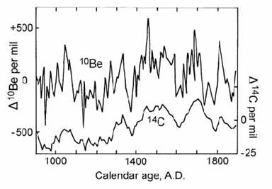
Fig. 14.27. Plot of 10Be variation in the South Pole ice core during a 1000 yr period from ca. 1900 to 900 compared with age-corrected 14C levels in tree rings. After Bard et al. (1997).
In contrast to the successful use of ice core material to study solar modulation of cosmogenic nuclide production, attempts to use ice core records of 10Be to chart geomagnetic modulation of cosmogenic production were much less successful. For example, a reconnaissance study of the long Dome C core (Raisbeck et al., 1981a) revealed a strong correlation of 10Be with *18O, which was attributed to the climatic effect of the last ice age. No significant correlation was observed with geomagnetic field strength, which reached a minimum value 6000 years ago and is argued to control long-term 14C variations. Yiou et al. (1985) suggested a partial solution to this problem by attributing the 10Be maximum during the last glaciation to lower precipitation at that time. This would sweep the same amount of 10Be out of the atmosphere, but concentrate it in a lower volume of ice, causing the 10Be record to be compressed.
The long-term Antarctic Dome C data were again matched by results from Camp Century in Greenland (Fig. 14.28). Beer et al. (1988) suggested two alternatives to explain the lack of correlation between the 10Be and geomagnetic intensity data. One idea was that 10Be ice-core data are recorded at high latitudes where the field strength has a weak influence on atmospheric cosmic-ray intensity. A more radical suggestion was that the long-term 10Be and 14C activity variations are not actually caused by geomagnetic field changes, but by a complex interplay of climatic effects and solar cosmic-ray modulations. However, more recent U)Th calibration of the radiocarbon time-scale (section 14.1.5) suggests that 14C variations up to 30 kyr old can largely be explained by variations in the Earth’s magnetic field. Hence, the ‘climate’ modulation theory is now largely discredited (but see section 14.3.4).
Fig. 14.28. Plot of 10Be and *18O variations in the Camp Century ice core (Greenland) over a depth of 1400 m, corresponding to ca. 10 kyr. After Beer et al. (1988).
It is now realised that the dramatic variations in 10Be abundance over the last glacial cycle are almost entirely a result of variable ice accumulation rates. Indeed, the method has more recently been used to chart paleo-accumulation rates in central Greenland, with a correction for variable atmospheric production based on geomagnetic field intensity data (Wagner et al., 2001). Such a correction would not be necessary if all of the 10Be signal was entirely local, since geomagnetic field intensity has little effect on cosmogenic production at the poles. Therefore, in order to study the effect of geomagnetic modulation of 10Be production, it is necessary to study equatorial production records from deep-sea sediments. These records are subject to perturbation by oceanic currents, but if these effects are quantified, suitable cores can yield reliable records of paleo 10Be production (section 14.3.4).
14.3.4 10Be in the oceans
Marine sediments were some of the first materials to be successfully analysed for 10Be, since they have concentrations measurable by $ counting. The objective was to use 10Be as a dating tool for oceanic sediments. However, early studies, which simply compared 10Be abundances at various depths with theoretical cosmogenic production rates, were unreliable. A more rigorous study was made by Tanaka and Inoue (1979) on paleomagnetically dated sediment cores from the Pacific ocean. These workers showed that absolute 10Be concentrations were variable from site to site, but that values at a given depth, relative to the sediment surface, were consistent with a theoretical decay path (Fig. 14.29). The good agreement between 10Be activities and a reference decay trajectory suggests that cosmogenic 10Be production has been constant to within about 30% over the last 2.5 Myr.
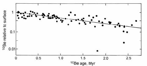
Fig. 14.29. Compilation plot of 10Be activity (normalized relative to the sediment surface) against burial age (depth) for five cores from the North Pacific. After Tanaka and Inoue (1979).
An important application of 10Be as a dating tool has been in studies of ferromanganese crusts. These deposits represent an ideal archive for particle-reactive species in the ocean system, such as Nd and Pb (section 4.5). Because the crusts grow into free space, they are resistant to contamination by clastic sediment particles and can accurately record long-term seawater isotope variations, provided their growth rates are accurate. For the past 500 kyr, the dating of crusts can be performed using U-series isotopes (section 12.3.2), but beyond the range of this method, 10Be is the best technique. This was first applied by Turekian et al. (1979) and is now used as a standard technique in oceanographic paleo tracer analysis (section 4.5.3).
Early studies of the behavior of stable 9Be in the oceans suggested that it was one of the classes of elements that very quickly precipitates from seawater (Merrill et al., 1960). This implies that fine particulates are the principal carrier of 10Be. This model was tested by Tanaka and Inoue (1979) by plotting the 10Be precipitation rate against the sedimentation rate at different sites in the Pacific (Fig. 14.30). The good positive correlation displayed by most of the data suggests that the particulate model is valid. Therefore, the net 10Be deposition flux at any given locality is dependent on the sedimentation rate rather than the cosmogenic flux. 10Be deposition rates are actually seen to vary by a factor of three above and below the theoretically predicted flux from the atmosphere. These variations in the 10Be depositional flux at different localities were attributed by Tanaka and Inoue to the lateral transport (advection) of fine particulates by ocean currents.
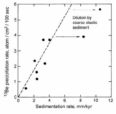
Fig. 14.30. Plot of 10Be precipitation rate against particulate sedimentation rate for the different Pacific Ocean sites. The dashed line represents a constant 10Be concentration in different cores. Arrows show the effect of dilution by excess clastic material. After Tanaka and Inoue (1979).
A detailed understanding of the behaviour of 10Be in the aqueous system requires a consideration of the oceanic residence time. Merrill et al. (1960) estimated the residence time of beryllium using equation [14.4] (Goldberg and Arrhenius, 1958):
total oceanic inventory
residence time = ))))))))))))))) [14.4]
total rate of introduction
This equation holds for a steady-state (equilibrium) system, which is approximated if the flux is constant for three residence times. For 10Be the equation can conveniently be calculated per unit area:
total water column budget/unit area
residence time = ))))))))))))))))) [14.5]
supply flux/unit area
Merrill et al. determined a residence time for 9Be attached to particulate matter of only 150 yr, but they estimated a longer residence time of 570 yr for the dissolved beryllium budget.
The first estimate of the soluble 10Be budget of the oceans was made by Yokoyama et al. (1978) based on 10Be/9Be ratios in manganese nodules. By assuming that these incorporated dissolved beryllium directly from seawater and using published 9Be abundances in the oceans, they calculated the dissolved 10Be budget as 2 H 109 atoms/g. Almost identical concentrations were determined by Raisbeck et al. (1980) in the first direct 10Be determinations on deep ocean waters, but their estimated residence time (630 yr) differed markedly from that of Yokoyama et al. (1600 yr) due to the use of different cosmogenic flux estimates. Raisbeck et al. used their own estimate of the cosmogenic 10Be flux, based on one year’s rain from a single locality in France, uncorrected for re-suspension of soil. This can now be seen to be an overestimate. Using the theoretical production rate of Reyss et al. (1981), both studies lead to a soluble 10Be residence time in the oceans of ca. 1200 yr.
Arnold (1958) divided the behavior of elements such as beryllium in the oceanic system into three categories: soluble/sorbed ions, pelagic particulate-controlled ions, and inshore particulate-controlled ions. All three types of behaviour can be seen to control 10Be. Despite its tendency to be adsorbed onto particulates, dissolved 10Be has a longer residence time in the oceans than similar adsorbable species such as 230Th (section 12.3.2). This difference can be explained by a nutrient-like behavior in beryllium (Measures and Edmond, 1982). Profiles of dissolved beryllium concentration in Pacific Ocean water (Fig. 14.31) show strong depletion near the surface where beryllium is are adsorbed onto organic matter, but relative enrichment at depth due to the breakdown of dead organic matter (releasing Be) as it falls through the water column (Kusakabe et al., 1987). These Pacific Ocean data yield a deep water 10Be concentration of 2 H 109 atom/g which is in agreement with the earlier results quoted above. However, Atlantic ocean water displays a different signature which may reflect the large river water input into this ocean basin.
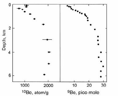
Fig. 14.31. Concentrations of dissolved 10Be (atom/g) and 9Be (pico Mole) are plotted as a function of water depth in the open ocean of the east Pacific. After Kusakabe et al. (1987).
The behavior of 10Be in the near-shore environment is very different from the open ocean, as proposed in Arnold’s model. Sediment cores from the continental rises off western Africa and western North America show 10Be accumulation rates at least an order of magnitude larger than the theoretical cosmogenic flux (Mangini et al., 1984; Brown et al., 1985). This is attributed to the advection of large quantities of 10Be by ocean currents into areas of high deposition. The high deposition rates may be caused by continental erosion or excess biological production, and in these localities, the transported 10Be is effectively scavenged and carried to the bottom.
Similar excess 10Be sedimentation rates have been seen in freshwater lakes (Raisbeck et al., 1981b). In this case, soil erosion in the drainage basin that supplied the lake caused the introduction of beryllium-rich sediment. Lundberg et al. (1983) proposed that the excess 10Be was introduced dominantly on the organic matter rather than silicate particles, consistent with the nutrient-like behavior of 10Be proposed for the oceanic system.
Comparisons between the Be isotope ratio of modern ocean masses were first made by Ku et al. (1990). These revealed a consistent global pattern of increasing 10Be/9Be ratio along the ocean conveyer belt, with values ranging from 0.6 H 10!7 in NADW, through 1 H 10!7 in the Antarctic, to values as high as 1.6 H 10!7 in deep Pacific water (Ku et al., 1990). This trend is shown in terms of increasing 10Be content with water age in Fig. 14.32. The positive trend is due to the low particulate sedimentation rate from NADW, which allows be 10Be to be advected to the Pacific, and implies a beryllium residence time similar to the circulation age of the ocean water masses. The precise residence time is difficult to constrain because of the different sources of the two isotopes: 10Be from global rain and 9Be from river water. However, the curve shown in Fig. 14.32 was modelled assuming a residence time of 600 yr (von Blankenburg et al. (1996).
Fig. 14.32. Plot of 10Be concentration against radiocarbon age in oceanic deep water to show the build-up of 10Be along the Ocean Conveyer Belt. ( ! ) = NADW; ( ” ) = Pacific deep water. After von Blankenburg et al. (1996).
Beryllium isotope ratios in the 10-7 range are less extreme than most cosmogenic isotope ratios, offering the possibility of analysis by conventional (non-accelerator) mass spectrometry. Such a method was developed by Belshaw et al. (1995) and applied by von Blankenburg et al. (1996) to the beryllium isotope analysis of ocean floor ferro-manganese crusts. Uranium isotope ratios were used to date the surface layer of the crust in order to apply an age correction in cases where the original growth surface had been removed by abrasion (section 12.3.2). Crusts of various ages (0 – 300 kyr) gave very consistent initial Be isotope ratios within each ocean basin, consistent with the beryllium composition of overlying deep ocean water. This suggests that the oceans have generally maintained the same circulation pattern over the past 300 kyr. However, more detailed comparisons of glacial and interglacial 10Be/9Be ratios are needed to test for any interruptions to the conveyer belt during glacial maxima.
14.3.5 Comparison of 10Be with other tracers
Ku et al. (1995) made the first comparison of 26Al and 10Be abundances in ocean water. They found 26Al/27Al ratios in surface water which were consistent with the expected 26Al flux from atmospheric production (by spallation of argon). Therefore, contributions of in situ cosmogenic 26Al from cosmic dust or wind-blown continental dust do not appear to be significant in sea water. However, the 26Al/10Be ratio measured in surface water was an order of magnitude lower than the atmospheric production ratio. This was therefore attributed to the much shorter ocean residence time of 26Al.
Wang et al. (1996) compared 26Al, 10Be and 230Th records in ocean floor sediments. The authigenic (seawater-derived) fractions of these nuclides were removed from core samples by leaching with NaOH. 10Be/9Be ratios in the leachates were in good agreement with the composition of overlying (North Pacific) deep water, whereas 10Be/9Be ratios in the bulk sediment were 50% lower, due to input from detrital continental beryllium. The 26Al budget in the sediment column was also in good agreement with the atmospheric production flux and with 26Al in ocean water (Ku, et al., 1995).
Comparison of authigenic 26Al, 10Be and excess initial 230Th revealed 26Al/230Th ratios consistent with the estimated production ratio, but excess abundances of 10Be relative to both the other nuclides (Fig. 14.33). Hence, it was concluded that 26Al and 230Th have similar (very short) residence times in ocean water, whereas the longer residence time of 10Be allows advection of 10Be into the North Pacific, where it is scavenged by high biogenic production. Similar effects are seen in the 231Pa/230Th system (section 12.3.6), but the effect on 10Be/26Al is larger, due to the longer ocean residence of 10Be. On the other hand, ratios of 231Pa/230Th are easier to measure, so both methods are likely to be very useful in paleo-oceanography.
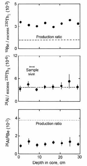
Fig. 14.33. Relative abundances of radionuclides in a sediment core from the North Pacific, showing ratios close to the production ratio for 26Al–230Th, but out of equilibrium with 10Be. After Wang et al. (1996).
Despite the complexities that may be introduced into 10Be sediment profiles by advection, marine sediments offer a better prospect than snow deposits for studying variations in paleo 10Be production. To overcome the problem of advection, Lao et al. (1992) compared 10Be abundances with the U-series nuclides 230Th and 231Pa. These nuclides have ocean chemistry similar to beryllium but are produced at a constant rate from uranium in solution. Lao et al. compared 10Be production at the present day and 20 kyr ago (corresponding to the last glacial maximum when the 14C flux was 140% of its present value). They normalized both 10Be and 231Pa fluxes against 230Th. However, based on a comparison of ocean residence times (section 12.3.6), we can best normalize climatic effects on 10Be deposition by comparing the 10Be/231Pa ratio at the present day and 20 kyr ago. After excluding one site with abnormal chemistry, 17 sites from the Pacific gave an average 10Be flux enhancement of 144% during the last glacial maximum, in excellent agreement with 14C.
Comparisons between the geomagnetic field strength and 10Be deposition have also been made by observing their variation over time in a single site. However, the existence of a direct (inverse) relationship between these variables depends on the neutralisation of climatic effects. In the absence of U-series data for normalisation, this may only happen by chance. Thus, Robinson et al. (1995) observed a good inverse relationship between 10Be and magnetic intensity in an 80 kyr old sediment core from the central North Atlantic. However, Raisbeck et al. (1994) observed no such relationship in a 600 – 800 kyr old section from the equatorial Pacific ocean (beyond the range of the 230Th dating method).
To avoid this type of problem, Frank et al. (1997) used only 230Th-dated cores to compile a global average of 10Be inventories for the past 200 kyr. This was based on 19 long cores which covered most of this age range, supplemented by 18 shorter cores covering the last 25 kyr. The global stack of 10Be abundance data (Fig. 14.34a) was then inverted to determine relative geomagnetic field intensity (Fig. 14.34b), which was found to correlate very well with a globally stacked paleointensity record (Fig. 14.34c).
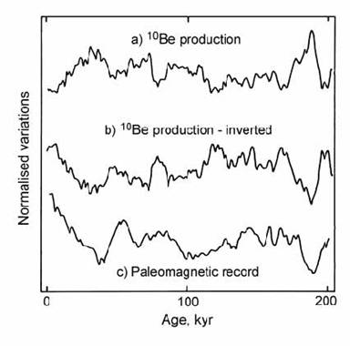
Fig. 14.34. Comparison between a global stack of 10Be paleointensity data (a, b) with a similar stack of magnetic paleointensity (c), demonstrating the paleomagnetic modulation of global cosmogenic isotope production. After Frank et al. (1997).
Kok (1999) expressed concern that both the 10Be and the paleointensity records might still not be completely free of climatically induced variations in sedimentation rate, despite the use of the 230Th dating method to calibrate the sections. This concern was prompted by the observation that the magnetic paleointensity record show a significant correspondence with the SPECMAP record of oxygen isotope variations (Fig. 14.35, a,b). However, two alternative explanations have since been offered for this correspondence. The first suggestion (Yamazaki and Oda, 2002) is that the geomagnetic field intensity is itself modulated by the Earth’s orbital eccentricity (which is thought to modulate climatic cycles). In that case, we would expect to see a correlation between variations in climate and the geomagnetic field. However, close examination of Fig. 14.35 shows that the 10Be-derived magnetic paleointensity stack (Fig. 14.35a) shows a stronger correspondence with the SPECMAP *18O record than the directly measured magnetic record. This suggests that it is the 10Be record, rather than the magnetic record, that contains a component with a climatic linkage.
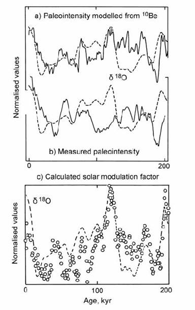
Fig. 14.35. Comparison of paleointensity record with the SPECMAP *18O record (dashed line). a) magnetic paleointensity derived from the inversion of 10Be data; b) directly measured magnetic paleointensity; c) normalized residual 10Be modulation attributed to solar field effects. After Kok (1999) and Sharma (2002).
Sharma (2002) examined this problem in more detail by extracting a residual 10Be modulation effect, after the subtraction of the geomagnetic modulation. This quantity was then normalized to its present-day value and is plotted in Fig. 14.35c along with the SPECMAP record. The controversial aspect of Sharma’s analysis was that he attributed the residual modulation effect to solar magnetic activity, which he suggested was also responsible for the 100 kyr glacial climate cycles during this period. This would then provide a ‘rival’ explanation for glacial cycles, relative to the widely accepted Milankovich model of ‘orbital tuning’ (section 12.4.2). The great success of the ‘astronomical timescale’ (section 10.4.2), obtained by orbital tuning of the oxygen isotope record, makes it hard to disbelieve the fundamental importance of the Milankovich model. However, there may be room for more than one influence on glacial cycles. Therefore, as one reviewer commented, Sharma’s model “could just be right”. Unfortunately, it will take time to accumulate the high quality 10Be and paleomagnetic records need to test this question further. In the meantime, it should be remembered that the Earth’s geomagnetic field is the principle modulating influence on cosmogenic isotope production.
14.3.6 10Be in magmatic systems
The most important application of 10Be as a petrogenetic tracer is in studies of the relationship between sediment subduction and island arc volcanism. In a reconnaissance study, Brown et al. (1982) demonstrated 10Be concentrations in island arc volcanics (2.7 H 106 ) 6.9 H 106 atom/g) which were generally much higher than the levels seen in a control group of continental and oceanic flood basalts. Brown et al. argued against high-level contamination of the analysed volcanics on the grounds that the short half-life of 10Be renders it extinct in all but surficial deposits, while 10Be levels in rain-water are too low to cause the observed enrichments. In contrast, it has long been known (e.g. Arnold, 1956) that pelagic sediments have very large 10Be contents, in excess of 109 atoms/g. Brown et al., therefore, attributed their data to the involvement of subducted ocean floor sediment in the genesis of island arc magmatism.
Subsequent studies (e.g. Tera et al., 1986) confirmed the general observation of high 10Be in island arc volcanics and low 10Be in the non-arc control group (Fig. 14.36). Detailed studies were also undertaken to assess the effects of weathering on the 10Be contents of lavas. Analyses of material collected during or immediately after eruption were shown to contain the same range of 10Be contents as historical lavas. Contamination of non-arc samples by radiogenic 10Be was only observed in severely altered samples. In situ cosmogenic production of 10Be in lavas at depths of 1 cm was also excluded, based on the low 10Be abundances in 16 Myr-old Columbia River basalts.
Fig. 14.36. Histograms of 10Be abundance in volcanic rocks. a) Non-arc control group and low-10Be arcs; b) high-10Be arcs. Symbols: A = sample from ‘active’ volcano; H = historic flow; F = fresh sample collected during or immediately after eruption. After Tera et al. (1986).
A surprising result of the detailed study of Tera et al. was that several arcs have 10Be levels as low as the maximum of 1 H 106 atoms/g in the control group. These included all samples from the Mariana, Halmahera (Moluccan) and Sunda arcs. To explain these observations, Tera et al. suggested four requirements for a positive 10Be signal in arc volcanics:
1) adequate 10Be inventory in trench sediments;
2) subduction rather than accretion of uppermost Be-enriched sediments;
3) incorporation of sediment in the magma source area;
4) transport time from sedimentation to magma source area < 10 Myr.
Failure of any one of these criteria could preclude a positive 10Be signal. However, Tera et al. did not observe simple correlations between 10Be and geophysical parameters such as age of the subducting plate.
In an attempt to harmonise their data from different arcs, Tera et al. plotted 10Be against a model parameter involving sedimentation rate, sediment thickness, plate velocity, and distance from trench to magma source. This quantity is specified as:
0o s | 8 l |
Predicted 10Be abundance = ))) exp – | ))) | [14.6]
8 h | v |
where 0o = 10Be abundance in the sediment, s = Plio)Pleistocene sedimentation rate, h = sediment thickness, l = the arc )trench gap, and v = plate velocity. Since the volcanic front is always located about 100 km above the seismic plane, the arc )trench gap is inversely proportional to the dip of the Benioff zone. Using this model, the contrast between the 10Be-rich Central American data and other arcs is explained by the high sedimentation rate and steep subduction angle of the former. However, both the Japanese and Aleutian arcs have a single 10Be-rich data point (shown by the dashed ranges in Fig. 14.37) which does not fit the model.
Fig. 14.37. Plot of 10Be data for seven arcs against a model parameter for the efficiency of 10Be supply to arc magma sources. 10Be signals are modelled for different bulk percentage sediment contributions to magmas. After Tera et al. (1986).
A further step in rationalising the 10Be systematics of arc volcanics was achieved by considering the data relative to non-cosmogenic (9Be) abundances (Monaghan et al., 1988; Morris and Tera, 1989). Within the different minerals of a single rock sample, 10Be is normally strongly correlated with total Be content (Fig. 14.38), implying that radiogenic and non-radiogenic Be were mixed before magmatic differentiation occurred. This further strengthens the arguments against surficial contamination of the lavas by 10Be, and also argues against crustal 10Be assimilation by magmas. Finally, the enriched Be contents of the groundmass, relative to phenocrysts, show that Be behaves as an incompatible element during magmatic differentiation.
Fig. 14.38. Plot of 10Be against total Be content for separated mineral phases, plus whole-rock (WR) and groundmass (GM) from two young lavas. Samples are from the Izalco volcano (Central America) and Akutan (Aleutians). After Morris and Tera (1989).
In contrast to Be mineral systematics, most whole-rock samples analysed by Morris and Tera did not show a strong correlation between 10Be and total Be. However, they did show a good correlation between 10Be/9Be ratios and absolute 10Be abundances (Fig. 14.39). These findings suggest that most of the rocks analysed, which were basalts, did not have their 10Be contents perturbed by magmatic differentiation. However, some andesites lie significantly to the right of the main trend, including the Japanese and Aleutian samples with abnormally high 10Be contents in Fig. 14.37 (Tera et al., 1986).
Fig. 14.39. Plot of 10Be/9Be against 10Be abundance for basalts ( ! ) and evolved rocks ( ” ) from different arc and non-arc environments. After Morris and Tera (1989).
Further constraints on the timing of subduction-related processes were obtained by combining 10Be/9Be and 238U/230Th data. Sigmarsson et al. (1990) observed that these ratios were correlated in the Southern Volcanic Zone of the Andes (section 13.4). Based on this correlation, and the much shorter half-life of 230Th than 10Be, Sigmarsson et al. suggested that the time-scale for dehydration, melting and eruption of these arc magmas was probably less than 20 kyr.
A further step in understanding subduction-zone processes was achieved by comparing 10Be/9Be and boron/beryllium ratios in arc lavas (Morris et al., 1990). Several arcs displayed a strong positive correlation between these two variables (Fig. 14.40), despite the fact that the two beryllium isotopes and boron have different distributions in the subducted slab. 10Be is concentrated in the uppermost sediment layers and diminishes rapidly downwards, 9Be is distributed throughout the sediment column, whereas B is principally concentrated in the hydrothermally altered basaltic crust. Hence, there is no a priori reason why these three species should display coherent behaviour in arc volcanics. The fact that they do behave coherently in widely separated volcanoes along the length of an arc suggested to Morris et al. a very thorough homogenisation mechanism for Be and B during the process of subduction-related magma genesis. While such a process could occur in the solid state, it is easiest to conceive of the mixing of fluids driven off from different parts of the subducted slab. The convergence of all of the correlation lines at the origin points to complete stripping out of all boron from the subduction zone, with no long-term residence of this element in the mantle.
Fig. 14.40. Plot of 10Be/9Be against elemental B/Be ratio, showing correlation lines for arc volcanics relative to possible mixing end-members. Numbered ticks denote calculated percentages of slab-derived fluids necessary to generate the observed arrays by contamination of the mantle source. After Morris et al. (1990).
The observed correlation between 10Be/9Be ratio and elemental B/Be ratio suggests that the latter may represent a useful proxy for the former. This is important because it widens the applicability of beryllium data. Firstly, the elemental B/Be ratio can be used as a tracer of the slab component in arcs with low subduction rates, where 10Be is extinct by the time of eruption. Secondly, elemental ratios can be measured with less sophisticated analytical equipment such as ICP)MS. These advantages were demonstrated by Edwards et al. (1993b) in a study of basaltic lavas from the Indonesian arc. Edwards et al. were able to combine B/Be ratios with other radiogenic isotope systems in order to uniquely specify the Pb, Sr and Nd isotope signatures of the slab-derived component, which was modelled by a 80%)20% mixture of basaltic crust and Indian Ocean sediment. This signature was also distinguishable from enriched and depleted reservoirs in the mantle wedge. The use of elemental B/Be data made these deductions possible despite the fact that 10Be abundances were at baseline, showing this nuclide to be extinct in the analysed lavas.
REFERENCES
Adkins, J. F. and Boyle, E. A. (1997). Changing atmospheric ) 14C and the record of deep water paleoventilation ages. Paleoceanography 12, 337–44.
Anderson, E. C. and Libby, W. F. (1951). World-wide distribution of natural radiocarbon. Phys. Rev. 81, 64)9.
Andree, M., Oeschger, H., Broecker, W., Beaven, N., Klas, M., Bonani, G., Hoffman, H. J., Suter, M., Woelfli, W. and Peng, T.-H. (1986). Limits on ventilation rates for the deep ocean over the last 12,000 years. Climate Dynamics 1, 53–62.
Andrews, J. N., Davis, S. N., Fabryka-Martin, J., Fontes, J. C., Lehmann, B. E., Loosli, H. H., Michelot, J-L., Moser, H., Smith, B. and Wolf, M. (1989). The in situ production of radioisotopes in rock matrices with particular reference to the Stripa granite. Geochim. Cosmochim. Acta 53, 1803)15.
Arnold, J. R. (1956). Beryllium-10 produced by cosmic rays. Science 124, 584)5.
Arnold, J. R. (1958). Trace elements and transport rates in the ocean. 2nd UN Conf. on Peaceful Uses of Atomic Energy 18, 344)6. IAEA.
Arnold, J. R. and Libby, W. F. (1949). Age determinations by radiocarbon content: Checks with samples of known age. Science 110, 678)80.
Bard, E., Arnold, M., Fairbanks, R. G. and Hamelin, B. (1993). 230Th)234U and 14C ages obtained by mass spectrometry on corals. Radiocarbon 35, 191)9.
Bard, E., Arnold, M., Hamelin, B., Tisnerat-Laborde, N. and Cabioch, G. (1998). Radiocarbon calibration by means of mass spectrometric 230Th/234U and 14C ages of corals: an updated database including samples from Barbados, Mururoa and Tahiti. Radiocarbon 40, 1085–92.
Bard, E., Arnold, M., Mangerud, J., Paterne, M., Labeyrie, L., Duprat, J., Melieres, M. A., Sonstegaard, E. and Duplessy, J. C. (1994). The North Atlantic atmosphere–sea surface 14C gradient during the Younger Dryas climatic event. Earth Planet. Sci. Lett. 126, 275–87.
Fink, D., Middleton, R., Klein, J. and Sharma, P. (1990). 41Ca measurement by accelerator mass spectrometry and applications. Nucl. Instr. Meth. in Phys. Res. B 47, 79)96.
Forbush, S. E. (1954). Worldwide cosmic-ray variations, 1937)1952. J. Geophys. Res. 59, 525)42.
Frank, M., Schwarz, B., Baumann, S., Kubik, P. W., Suter, M. and Mangini, A. (1997). A 200 kyr record of cosmogenic radionuclide production rate and geomagnetic field intensity from 10Be in globally stacked deep-sea sediments. Earth Planet. Sci. Lett. 149, 121–9.
Godwin, H. (1962). Half-life of radiocarbon. Nature 195, 984.
Goldberg, E. D. and Arrhenius, G. O. S. (1958). Chemistry of Pacific pelagic sediments. Geochim. Cosmochim. Acta 13, 153)212.
Goldstein, S. J., Lea, D. W., Chakraborty, S., Kashgarian, M. and Murrell, M. T. (2001). Uranium-series and radiocarbon geochronology of deep-sea corals: implications for Southern Ocean ventilation rates and the ocean carbon cycle. Earth Planet. Sci. Lett. 193, 167–82.
Goslar, T., Arnold, M., Tisnerat-Laborde, N., Czernik, J. and Wieckowski, K. (2000). Variations of Younger Dryas atmospheric radiocarbon explicable without ocean circulation changes. Nature 403, 877–80.
Gove, H. E. (1987). Tandem-accelerator mass-spectrometry measurements of 36Cl, 129I and osmium isotopes in diverse natural samples. Phil. Trans. Roy. Soc. Lond. A 323, 103)19.
Granger, D. E., Fabel, D. and Palmer, A, N. (2001). Pliocene–Pleistocene incision of the Green river, Kentucky, determined from radioactive decay of cosmogenic 26Al and 10Be in Mammoth Cave sediments. GSA Bulletin 113, 825–36.
Granger, D. E. and Muzikar, P. F. (2001). Dating sediment burial with in situ-produced cosmogenic nuclides: theory, techniques, and limitations. Earth Planet. Sci. Lett. 188, 269–81.
Hammer, C. U., Clausen, H. B. and Tauber, H. (1986). Ice-core dating of the Pleistocene/Holocene boundary applied to a calibration of the 14C time scale. Radiocarbon 28, 284)91.
Henning, W. (1987). Accelerator mass spectrometry of heavy elements: 36Cl to 205Pb. Phil. Trans. Roy. Soc. Lond. A 323, 87)99.
Hillam, J., Groves, C. M., Brown, D. M., Baillie, M. G. L., Coles, J. M. and Coles, B. J. (1990). Dendrochronology of the English Neolithic. Antiquity 64, 210)20.
Hofmann, H. J., Beer, J., Bonani, G., Von Gunten, H. R., Raman, S., Suter, M., Walker, R. L., Wolfli, W. and Zimmermann, D. (1987). 10Be half-life and AMS-standards. Nucl. Instr. Meth. in Phys. Res. B 29, 32)6.
Huber, B. (1970). Dendrochronology of central Europe. In: I. U. Olsson (Ed.), Radiocarbon Variations and Absolute Chronology, Proc. 12th Nobel Symp. Wiley, pp. 233)5.
Hughen, K. A., Overpeck, J. T., Lehman, S. J., Kashgarian, M., Southon, J., Peterson, L. C., Alley, R. and Sigman D. M. (1998). Deglacial changes in ocean circulation from an extended radiocarbon calibration. Nature 391, 65–8.
Kamen, M. D. (1963). Early history of carbon-14. Science 140, 584)90.
Key, R., Quay, P. D., Jones, G. A., McNichol, A. P., Von Reden, K. F. and Schneider, R. J. (1996). WOCE AMS radiocarbon I: Pacific Ocean results (P6, P16, P17). Radiocarbon 38, 425–518.
Kieser, W. E., Beukens, R. P., Kilius, L. R., Lee, H. W. and Litherland, A. E. (1986). Isotrace radiocarbon analysis ) equipment and procedures. Nucl. Instr. Meth. in Phys. Res. B 15, 718)21.
Kitagawa, H. and van der Plicht, J. (1998). Atmospheric radiocarbon calibration to 45,000 yr B.P.: Late glacial fluctuations and cosmogenic isotope production. Science 279, 1187–90.
Klein, J., Fink, D., Middleton, R., Nishiizumi, K. and Arnold, J. (1991). Determination of the half-life of 41Ca from measurements of Antarctic meteorites. Earth Planet. Sci. Lett. 103, 79)83.
Kok, Y. S. (1999). Climatic influence in NRM and 10Be-derived geomagnetic paleointensity data. Earth Planet. Sci. Lett. 166, 105–19.
Ku, T. L., Wang, L., Luo, S. and Southon, J. R. (1995). 26Al in seawater and 26Al/10Be as paleo-flux tracer. Geophys. Res. Lett. 22, 2163–6.
Ku, T. L., Kusakabe, M., Measures, C. I., Southon, J. R., Cusimano, G., Vogel, J. S., Nelson, D. E. and Nakaya, S. (1990). Beryllium isotope distribution in the western North Atlantic: a comparison to the Pacific. Deep-Sea Res. 37, 795–808.
Kusakabe, M., Ku, T. L., Southon, J. R., Vogel, J. S., Nelson, D. E., Measures, C. I. and Nozaki, Y. (1987). The distribution of 10Be and 9Be in ocean water. Nucl. Instr. Meth. in Phys. Res. B 29, 306)10.
Labrie, D. and Reid, J. (1981). Radiocarbon dating by infrared laser spectroscopy. Appl. Phys. 24, 381)6.
Lal, D. (1988). In situ-produced cosmogenic isotopes in terrestrial rocks. Ann. Rev. Earth Planet. Sci. 16, 355)88.
Lal, D. and Peters, B. (1967). Cosmic-ray produced radioactivity on the Earth. In: Handbook of Physics. 46/2. Springer, pp. 551)612.
Lao, Y., Anderson, R. F., Broecker, W. S., Trumbore, S. E., Hofmann, H. J. and Wolfli, W. (1992). Increased production of cosmogenic 10Be during the Last Glacial Maximum. Nature 357, 576–8.
Lee, H. W., Galindo-Uribarri, A., Chang, K. H., Kilius, L. R. and Litherland, A. E. (1984). The 12CH2+2 molecule and radiocarbon dating by accelerator mass spectrometry. Nucl. Instrum. Meth. in Phys. Res. B 5, 208)10.
Libby, W. F. (1952). Radiocarbon Dating. University of Chicago Press, 124 p.
Libby, W. F. (1970). Ruminations on radiocarbon dating. In: I. U. Olsson (Ed.), Radiocarbon Variations and Absolute Chronology, Proc. 12th Nobel Symp. Wiley, pp. 629)40.
Litherland, A. E. (1980). Ultra-sensitive mass spectrometry with accelerators. Ann. Rev. Nucl. Part. Sci. 30, 437)73.
Litherland, A. E. (1987). Fundamentals of accelerator mass spectrometry. Phil. Trans. Roy. Soc. Lond. A 323, 5)21.
Liu, B., Phillips, F. M., Fabryka-Martin, J. T., Fowler, M. M. and Stone, W. D. (1994). Cosmogenic 36Cl accumulation in unstable landforms 1. effects of the thermal neutron distribution. Water Resour. Res. 30, 3115–25.
Lundberg, L., Ticich, T., Herzog, G. F., Hughes, T., Ashley, G., Moniot, R. K., Tuniz, C., Kruse, T. and Savin, W. (1983). 10Be and Be in the Maurice River ) Union Lake system of Southern New Jersey. J. Geophys. Res. 88, 4498)504.
Mangini, A., Segl, M., Bonani, G., Hofmann, H. J., Morenzoni, E., Nessi, M., Suter, M., Wolfli, W. and Turekian, K. K. (1984). Mass-spectrometric 10Be dating of deep-sea sediments applying the Zurich tandem accelerator. Nucl. Instr. Meth. in Phys. Res. B 5, 353)8.
Marchal, O., Stocker, T. F. and Muschler, R. (2001). Atmospheric radiocarbon during the Younger Dryas: production, ventilation, or both? Earth Planet. Sci. Lett. 185, 383–95.
Mazaud, A., Laj, C., Bard, E., Arnold, M. and Tric, E. (1991). Geomagnetic field control of 14C production over the last 80 kyr: implications for the radiocarbon time-scale. Geophys Res. Lett. 18, 1885)8.
McCorkell, R., Fireman, E. L. and Langway, C. C. (1967). Aluminium-26 and Beryllium-10 in Greenland Ice. Science 158, 1690)2.
Measures, C. I. and Edmond, J. M. (1982). Beryllium in the water column of the central North Pacific. Nature 297, 51)3.
Merrill, J. R., Lyden, E. F. X., Honda, M. and Arnold, J. R. (1960). The sedimentary geochemistry of the beryllium isotopes. Geochim. Cosmochim. Acta 18, 108)29.
Middleton, R. and Klein, J. (1987). 26Al: measurement and applications. Phil. Trans. Roy. Soc. Lond. A 323, 121)43.
Mitchell, S. G., Matmon, A., Bierman, P. R., Enzel, Y., Caffee, M. and Rizzo, D. (2001). Displacement history of a limestone normal fault scarp, northern Israel, from cosmogenic 36Cl. J. Geophys. Res. 106, 4247–64.
Monaghan, M. C., Klein, J. and Measures, C. I. (1988). The origin of 10Be in island-arc volcanic rocks. Earth Planet. Sci. Lett. 89, 288)98.
Mook, W. G. (1986). Business meeting: Recommendations/resolutions adopted by the Twelfth International Radiocarbon conference. Radiocarbon 28, 799.
Mook, W. G. and Streurman, H. J. (1983). Physical and chemical aspects of radiocarbon dating. P.A.C.T. (Physical And Chemical Techniques in Archaeology) 8, 31)55.
Morris, J. D., Leeman, W. P. and Tera, F. (1990). The subducted component in island arc lavas: constraints from Be isotopes and B)Be systematics. Nature 344, 31)6.
Phillips, F. M., Bentley, H. W., Davis, S. N., Elmore, D. and Swanick, G. B. (1986). Chlorine 36 dating of very old groundwater 2. Milk River aquifer, Alberta, Canada. Water Resour. Res. 22, 2003)16.
Phillips, F. M., Leavy, B. D., Jannik, N. O., Elmore, D. and Kubik, P. W. (1986). The accumulation of cosmogenic chlorine-36 in rocks: a method for surface exposure dating. Science 231, 41–3.